Timing experiments

In this note we describe the experiments we performed so as to time synchronisation constructs.

The complete sources and logs are available, for x86 X86-SPEED (archive) and Power PPC-SPEED (archive).

Contents

• 1  Generating tests
• 2  Running the tests
• 3  Measures
  • 3.1  x86
  • 3.2  Power

1  Generating tests

We build series of 8 tests named X01 to X08 involving from 1 to 8 threads. The code of each thread consists in a write to location, as x_i and a read from location say x_i+1 (the read of the last thread being from x₁). In practice we generate the tests with diyone. For instance X03 for x86 is produced by:

% diyone -arch X86 -name X03 PodWR Fre PodWR Fre PodWR Fre

While X03 for Power is produced by:

% diyone -arch PPC -name X03 PodWR Fre PodWR Fre PodWR Fre

Note that the first test of a batch (X01 for x86 and X01 for Power) is written by hand, as it cannot be induced by a cycle of candidate relaxations. We then build series of synchronised tests, either with offence or by hand.

For x86 from the batch ’X’, we produce three batches:

• ’F’ by running offence -technique fence, see for instance F03, for timing mfence;
• ’A’ by running offence -technique atom, see for instance A03, for timing xchg;
• ’L’ by running offence -technique lock, see for instance L03, for timing locks.

Notice that in the case of locks, there are two LOCK/UNLOCK sequences per thread, to different lock variables. The alternative of one LOCK/UNLOCK sequence per thread would result in less concurrent execution and has not been tested.

For Power from the batch ’X’, we produce four batches:

• ’F’ by running offence -technique fence, see for instance F03, for timing sync;
• ’W’ by changing the sync instructions of batch ’F’ into lwsync¹ instructions, see for instance W03, for timing lwsync;
• ’A’ by running offence -technique atom, see for instance A03, for timing STA/FNO pairs;
• ’L’ by running offence -technique lock, see for instance L03, for timing locks.

2  Running the tests

In the previous, soundness, experiment, the test harness of litmus accounted for an important part of running times. In this experiment we minimise the impact of harness code by:

1. running test code only once, with litmus options -a 1 -s 1 -r 1;
2. and inserting the code of each thread of tests in a loop of size 100 · 10⁶, with litmus option -loop 100M.

We perform these settings with litmus configuration file speed.cfg.

The altered test code can be seen in litmus logs, for instance here is the code actually executed by the first thread of F03:

...
 P0          | P1          | P2          ;
 MOV [z],$1  | MOV [x],$1  | MOV [y],$1  ;
 MFENCE      | MFENCE      | MFENCE      ;
 MOV EAX,[x] | MOV EAX,[y] | MOV EAX,[z] ;
...
 _litmus_P0_0_: cmpl $0,%edx
 _litmus_P0_1_: jmp Lit__L1
 _litmus_P0_2_: Lit__L0:
 _litmus_P0_3_: movl $1,(%r8)
 _litmus_P0_4_: mfence
 _litmus_P0_5_: movl (%r9),%eax
 _litmus_P0_6_: decl %edx
 _litmus_P0_7_: Lit__L1:
 _litmus_P0_8_: jg Lit__L0
...

Where %edx is the loop counter. We run all test batches at least five times on our 8 core machines, chianti for x86 and power7 for Power.

3  Measures

3.1  x86

We get the log files C.00 to C.04, of which we extract the following timings (times are wall-clock times of a test run, in seconds):

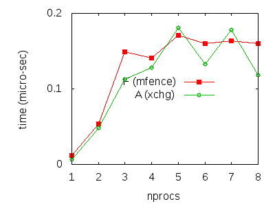
So as to approximate the time taken by one synchronisation construct, we first select a value for each test, taking the median of the five measures performed. Then, we subtract the value found for a given ’X’ test from the corresponding ’F’, ’A’ or ’L’ values and divide the result by iteration size (10⁸). The final numbers are decent approximations of synchronisation costs. We plot them below, including and excluding the plot for the mapping ’L’:

Such time measures are to be treated with caution, due to the non-determinism of the test itself, to the intervention of the system scheduler etc. However, we argue that we can draw a few conclusions from them:

1. Locks are much more expensive than fences and atomic exchange.
2. While fast in isolation (nproc=1), fences and atomic exchange get more expensive by a factor of at least ten when communication by shared memory indeed occurs.
3. mfence and xchg incur similar time penalties.

3.2  Power

We get the log files P.00 to P.04 and P.10 to P.14, of which we extract the following timings (times are wall-clock times, in seconds):

Times for batch ’W’ (lwsync) are from different runs:

We compute approximations of synchronisation cost as we did for x86:

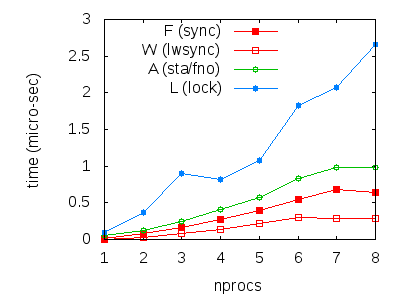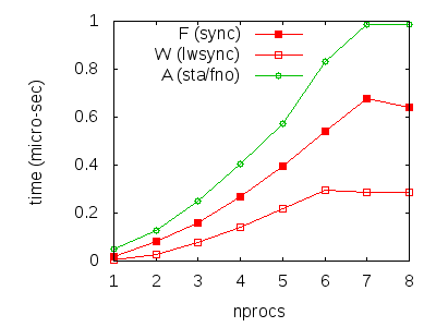Again, our numbers are to be treated with caution. However, we can draw a few conclusions from them:

1. Locks are more expensive than fences and atomic pairs.
2. While fast in isolation (nproc=1), fences and atomic pairs get more expensive by a factor of at least ten when communication by shared memory indeed occurs.
3. lwsync, sync and sta/fno incur increasing time penalties, both from lwsync to sta/fno and as the number of processors involved grows.

Complete sources and logs: for x86 X86-SPEED (archive) and Power PPC-SPEED (archive).

1

A lwsync fence between a store and a load is useless. However this is irrelevant to our purpose of measuring its cost, as we checked with similar examples on store-store pairs.

This document was translated from L^AT_EX by H^EV^EA.